| Wood Anderson Seismometer
- Calibration (.pdf) | ||||||||||||||||||||||||||
|
Following the refurbishment, in 2002 the TS-220 instruments were disassembled, cleaned, and completely recalibrated according to the maintenance manual.
Some adjustment screws located on the base of the instrument housing
(Fig.2a, Fig.2b)
allowed the instrument to tilt, thus affecting the gravity component acting on the mass. Changing the tilt enabled us to adjust the seismometer’s natural period.
The value of the damping was recalibrated to obtain a value
that is as close as possible to the theoretical damping (h= 0.8). The period and the damping values obtained after the 2002 calibration of the TS-220
are reported in Table 1. The trace amplitude recorded by the new digital acquisition system
of the TS-220 is given in counts. To compute the factor to convert counts into millimeters, we manually moved a needle between two marks located on the base of the instrument
case and read the corresponding counts (Fig.2a). We repeated this operation several times to obtain
a mean value of counts corresponding to the needle movements. In the original WA,
moving the needle between the two marks corresponded to a 100 mm displacement on the photographic paper. Therefore, the conversion factor is computed
as the ratio between 100 mm and the mean value of the counts, and its error is the standard deviation of the distribution of the peaks in counts.
| ||||||||||||||||||||||||||
 |
 |
|||||||||||||||||||||||||
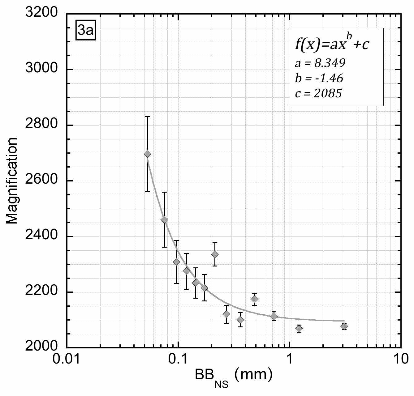
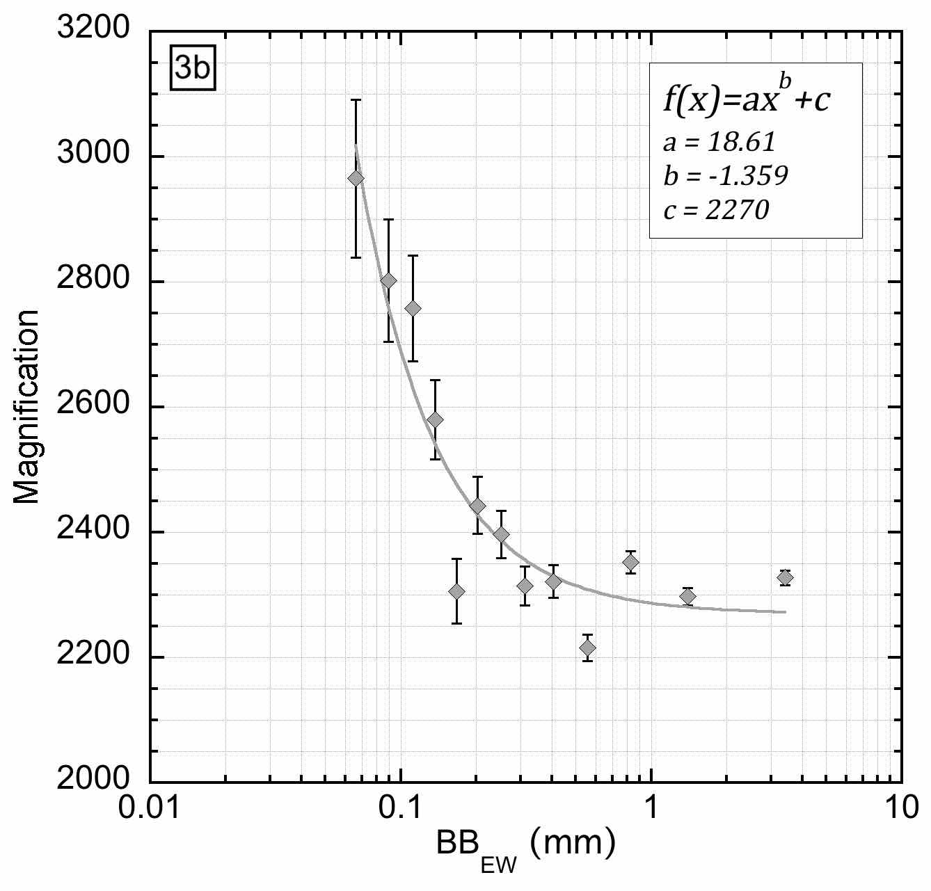
| WA static magnification (Gs) versus amplitude of the broadband (BB) seismograms recorded on the (a) north–south (NS) and (b) east–west (EW) components. | ||||||||||||||||||||||||||
|
Anderson and Wood (1925) determined a magnification value of 2800 for their instrument, but in doing so they neglected the deformation of the
taut tungsten wire from a straight line due to the catenary effect. In fact, the deformation of the wire could be sufficient to reduce the
magnification by a factor of 0.3 due to the increase in the polar moment of inertia of the copper cylinder. For this reason, when Uhrhammer
and Collins (1990) and Uhrhammer et al. (1996) carefully computed the static magnification (Gs) of the instrument at Berkeley, California,
they found Gs to be equal to 2080 +/- 60. Using 2800 instead of 2080 in the BB WA simulations leads to a mag- nitude difference of +0.129 (e.g.,
Uhrhammer et al., 2011). To verify the Gs value of the Trieste instrument, we adopted two different approaches. The first approach involves a
direct action on the instrument. According to Anderson and Wood (1925), Gs is determined by Gs=A/a=L/l=4π^2A/gbT0^2 in which A is the seismogram trace
amplitude, a is the amplitude of the ground-motion component normal to the equilibrium plane, l is the mass swinging center distance from
the rotation axis, L is the optical lever length, g is the gravitational acceleration, b is the instrument tilt angle (in radians), and T0 is
the period of oscillation of the instrument (ideally 0.8 s). Tilting the instrument by a known angle b and measuring the output voltage from
the PSD, which is proportional to A, equation (1) allowed us to calculate Gs (Table 1).
The error associated with the estimate of Gs is evaluated
considering that the amplifier error is 1% on the linearity of the response, and the accuracy of the voltmeter is equal to 0.05 V. The second
method to check Gs is based upon a comparison of the maximum peak of the seismograms recorded by the WA and Güralp 40-T BB instruments that
are placed side by side (LINK). Hereinafter we use “amplitude” to mean the trace amplitude in millimeters that we would have obtained
with the original recording system. We first sorted the values of the WA amplitudes in ascending order; using a sliding window of 50 WA samples,
we calculated the Gs values as the weighted average of the ratios between the WA and BB peak amplitudes (Fig. 3a and 3b, corresponding to north–
south and east–west components, respectively). In this test, the BB waveforms were corrected for instrument response to simulate the WA but using
a static magnification equal to 1. The weights are given by the inverse of the uncertainty on each peak, which is a function of the conversion
factor error of the system and the 1% error of the amplifier. We observe that the trends of the values obtained for the north–south component
(Fig.3a)
and for the east–west component (Fig.3b), respectively, are slightly different.
This is probably because the east–west component was repaired by
the OGS technical staff after a partial detachment of the moving mirror, which could have affected somehow the accuracy of the orientation of the
mirror with respect to the wire. However, we observe that the Gs values on both components decrease with increasing amplitude
(Fig.3a,b):
for amplitudes >1 mm they tend asymptotically to 2080, which is the value calculated by Uhrhammer and Collins (1990), suggesting the results of
Uhrhammer and Collins are only valid for larger amplitudes. For an amplitude value of 0.05 mm, Gs is close to 2800. The value obtained for large
amplitudes is very similar to that obtained by the first method (see Table 1).
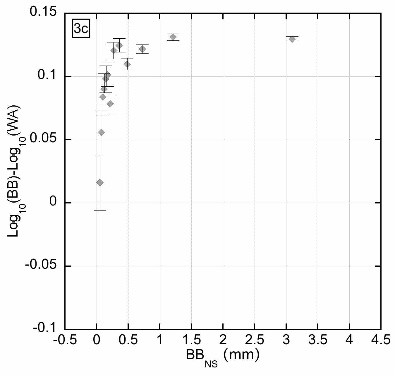
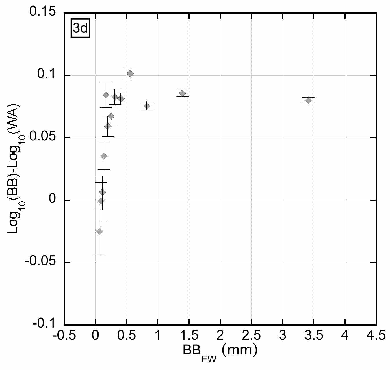
Figure 3c,d
show the difference between the equivalent ML estimated
by a BB record with Gs equal to 2800 and the ML estimated by the WA seismograph. Fixing Gs equal to 2800, we compute an error in magnitude that,
depending on the recorded peak amplitudes, spans from 0 for smaller amplitudes to 0.13 for amplitudes >0:05 mm.
| ||||||||||||||||||||||||||
 |
 |
|||||||||||||||||||||||||
| The error in magnitude estimation due
to setting Gs equal to 2800 is plotted as a function of the amplitude of the waveforms recorded on the (c) N-S and (d) E-W components.
|
||||||||||||||||||||||||||
| References to info-rts@inogs.it | ||||||||||||||||||||||||||